Acceleration

[OpenStax College physics 2e: Kinematics] One-dimensional motion: Basic concepts

Acceleration

In everyday conversation, to accelerate means to speed up. The accelerator in a car can in fact cause it to speed up. The greater the acceleration, the greater the change in velocity over a given time. The formal definition of acceleration is consistent with these notions, but more inclusive.

Average acceleration

Average acceleration is the rate at which velocity changes,

\[ \begin{array}{rcl}\blue{\bar{a}}&=&\dfrac{\green{\Delta v}}{\orange{\Delta t}}&=&\dfrac{\green{{v}_{f}}-\green{{v}_{0}}}{\orange{{t}_{f}}-\orange{{t}_{0}}}\end{array}\]

where #\blue{\bar{a}}# is average acceleration, #\green{v}# is velocity, and #\orange{t}# is time (the bar over the #\blue{a}# means average acceleration and recall that the subscripts #f# and #0# mean final and initial respectively).

Units

Because acceleration is velocity in #\rm{m/s}# divided by time in #\rm{s}#, the SI units for acceleration are #{\mathrm{\ m/s}}^{2}#, meters per second squared or meters per second per second, which literally means by how many meters per second the velocity changes every second.

Recall that velocity is a vector, i.e., it has both magnitude and direction. This means that a change in velocity can be a change in magnitude (or speed), but it can also be a change in direction. For example, if a car turns a corner at constant speed, it is accelerating because its direction is changing. The quicker you turn, the greater the acceleration. So there is an acceleration when velocity changes either in magnitude (an increase or decrease in speed) or in direction, or both.

Acceleration as a vector

Acceleration is a vector in the same direction as the change in velocity, #\green{\Delta v}#. Since velocity is a vector, it can change either in magnitude or in direction. Acceleration is therefore a change in either speed or direction, or both.

Deceleration

Keep in mind that although acceleration is in the direction of the change in velocity, it is not always in the direction of motion. When an object slows down, its acceleration is opposite to the direction of its motion. This is known as deceleration.

Misconception alert: deceleration vs. negative acceleration

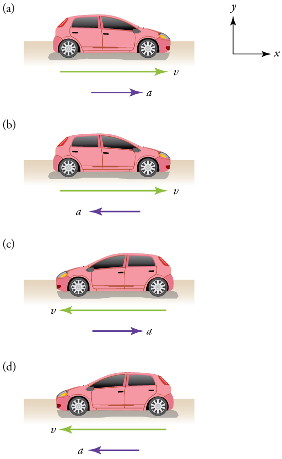
Deceleration always refers to acceleration in the direction opposite to the direction of the velocity. Deceleration always reduces speed. Negative acceleration, however, is acceleration in the negative direction in the chosen coordinate system. Negative acceleration may or may not be deceleration, and deceleration may or may not be considered negative acceleration. For example, consider Figure 1.

Fig. 1 (a) This car is speeding up as it moves toward the right. It therefore has positive acceleration in our coordinate system. (b) This car is slowing down as it moves toward the right. Therefore, it has negative acceleration in our coordinate system, because its acceleration is toward the left. The car is also decelerating: the direction of its acceleration is opposite to its direction of motion. (c) This car is moving toward the left, but slowing down over time. Therefore, its acceleration is positive in our coordinate system because it is toward the right. However, the car is decelerating because its acceleration is opposite to its motion. (d) This car is speeding up as it moves toward the left. It has negative acceleration because it is accelerating toward the left. However, because its acceleration is in the same direction as its motion, it is speeding up (not decelerating).

As with velocity, it is possible to take the time interval used to obtain the average acceleration to be infinitesimally small, thus obtaining the instantaneous acceleration. While such computations are outside the scope of this text, we will make use of the concept of instantaneous acceleration.

Instantaneous acceleration

Instantaneous acceleration, #\blue{a}#, or the acceleration at a specific instant in time, is obtained by the same process as discussed for instantaneous velocity in Time, velocity, and speed; that is, by considering an infinitesimally small interval of time. How do we find instantaneous acceleration using only algebra? The answer is that we choose an average acceleration that is representative of the motion.

Let us look at an example of how to select an average acceleration from a graph of the instantaneous acceleration over time.

Example

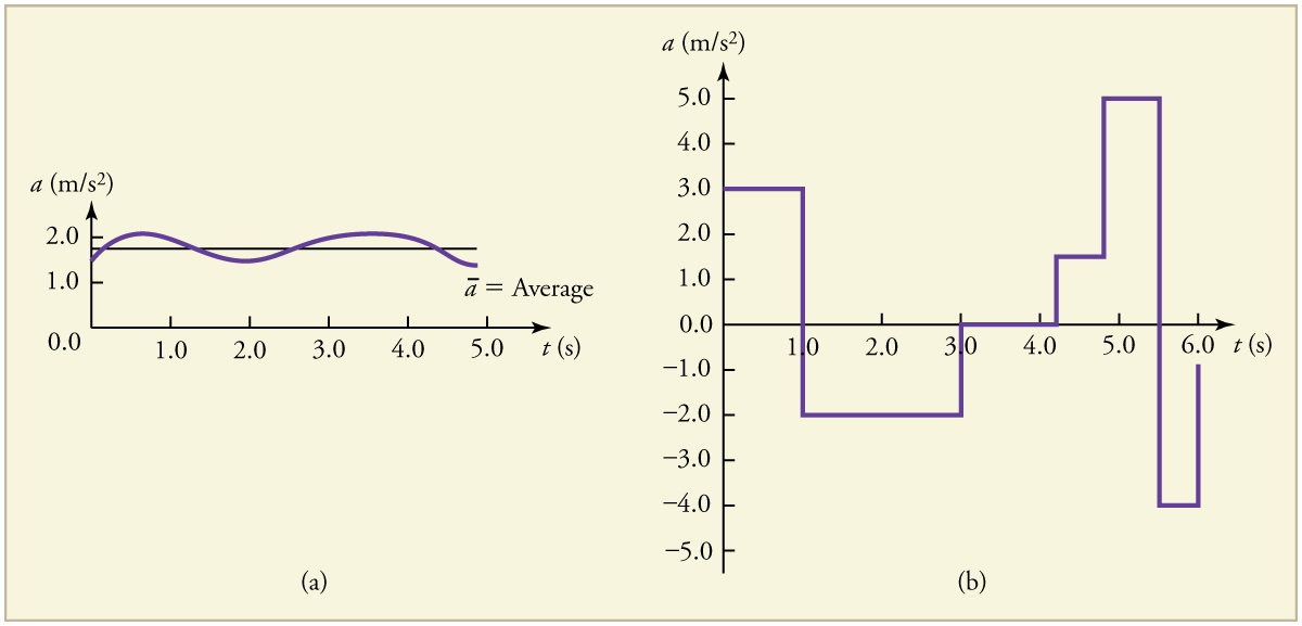
Figure 2 shows graphs of instantaneous acceleration versus time for two very different motions. In Figure 2 (a), the acceleration varies slightly and the average over the entire interval is nearly the same as the instantaneous acceleration at any time. In this case, we should treat this motion as if it had a constant acceleration equal to the average (in this case about #\blue{\unit{1.8}{m/s^2}}#). In Figure 2 (b), the acceleration varies drastically over time. In such situations it is best to consider smaller time intervals and choose an average acceleration for each. For example, we could consider motion over the time intervals from #\orange{0}# to #\orange{\unit{1.0}{s}}# and from #\orange{1.0}# to #\orange{\unit{3.0}{s}}# as separate motions with accelerations of #\blue{\unit{+3.0}{ m/s^2}}# and #\blue{\unit{–2.0}{ m/s^2}}#, respectively.

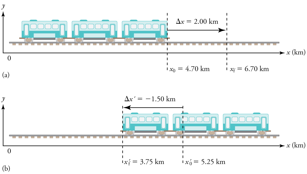
Fig. 2 Graphs of instantaneous acceleration versus time for two different one-dimensional motions. (a) Here acceleration varies only slightly and is always in the same direction, since it is positive. The average over the interval is nearly the same as the acceleration at any given time. (b) Here the acceleration varies greatly, perhaps representing a package on a post office conveyor belt that is accelerated forward and backward as it bumps along. It is necessary to consider small time intervals (such as from #\orange{0}# to #\orange{\unit{1.0}{s}}#) with constant or nearly constant acceleration in such a situation.

The next several examples consider the motion of the subway train shown in Figure 3. In (a) the shuttle moves to the right, and in (b) it moves to the left. The examples are designed to further illustrate aspects of motion and to illustrate some of the reasoning that goes into solving problems.

Fig. 3 One-dimensional motion of a subway train considered in the examples below. Here we have chosen the #x#-axis so that #+# means to the right and #-# means to the left for displacements, velocities, and accelerations. (a) The subway train moves to the right from #{x}_{0}# to #{x}_{f}#. Its displacement #\Delta x# is #\unit{+2.0}{km}#. (b) The train moves to the left from #{x'}_{0}# to #{x'}_{f}#. Its displacement #\Delta x'# is #\unit{-1.5}{km}# (note that the prime symbol (′) is used simply to distinguish between displacement in the two different situations. The distances of travel and the size of the cars are on different scales to fit everything into the diagram).

Calculating displacement: a subway train

What are the magnitude and sign of displacements for the motions of the subway train shown in parts (a) and (b) of Figure 3?

1. Outline a strategy

A drawing with a coordinate system is already provided, so we don’t need to make a sketch, but we should analyze it to make sure we understand what it is showing. Pay particular attention to the coordinate system. To find displacement, we use the equation #\Delta x={x}_{f}-{x}_{0}#. This is straightforward since the initial and final positions are given.

2. Solve for the displacement

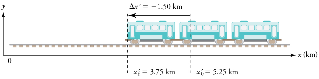
Identify the knowns. In the figure we see that #{x}_{f}=\unit{6.70}{km}# and #{x}_{0}=\unit{4.70}{km}# for part (a), and #{x'}_{f}=\unit{3.75}{ km}# and #{x'}_{0}=\unit{5.25}{km}# for part (b).
Solve for displacement in part (a).
\[ \Delta x={x}_{f}-{x}_{0}=6.70-4.70=\unit{+2.00}{km} \]
Solve for displacement in part (b).
\[ \Delta x' ={x' }_{f}-{x'}_{0}=3.75 -5.25 = \unit{-1.50}{km}\]

Discussion

The direction of the motion in (a) is to the right and therefore its displacement has a positive sign, whereas motion in (b) is to the left and thus has a negative sign.

New example

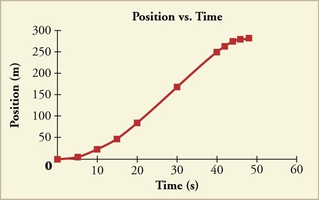
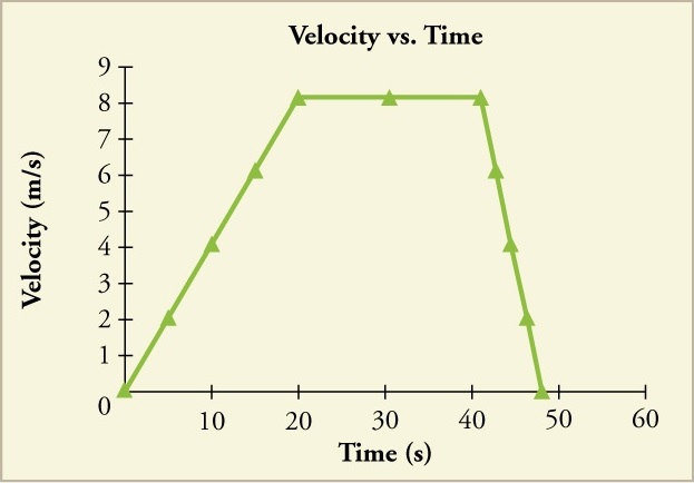
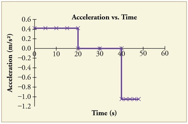
The graphs of position, velocity, and acceleration vs. time for the trains in the examples above and below are displayed in Figure 6 (we have taken the velocity to remain constant from #\orange{20}# to #\orange{\unit{40}{s}}#, after which the train decelerates).

Fig. 6 (a) Position of the train over time. Notice that the train’s position changes slowly at the beginning of the journey, then more and more quickly as it picks up speed. Its position then changes more slowly as it slows down at the end of the journey. In the middle of the journey, while the velocity remains constant, the position changes at a constant rate. (b) Velocity of the train over time. The train’s velocity increases as it accelerates at the beginning of the journey. It remains the same in the middle of the journey (where there is no acceleration). It decreases as the train decelerates at the end of the journey. (c) The acceleration of the train over time. The train has positive acceleration as it speeds up at the beginning of the journey. It has no acceleration as it travels at constant velocity in the middle of the journey. Its acceleration is negative as it slows down at the end of the journey.

Calculating average velocity: the subway train

What is the average velocity of the train of Figure 3 (b), and shown again below, if it takes #\unit{5.00}{min}# to make its trip?

Fig. 7 The train moves to the left from #{x'}_{0}# to #{x'}_{f}#. Its displacement #\Delta x'# is #\unit{-1.5}{km}#.

1. Outline a strategy

Average velocity is displacement divided by time. It will be negative here, since the train moves to the left and has a negative displacement.

2. Solve for the velocity

Identify the knowns. #{x' }_{f}=\unit{3.75}{km}#, #{x'}_{0}=\unit{5.25}{km}#, #\Delta t=\unit{5.00}{min}#.
Determine displacement, #\Delta x' #. We found #\Delta x' # to be #\unit{-1.5}{km}# in an example above.
Solve for average velocity.
\[ \bar{v}=\dfrac{\Delta x' }{\Delta t}=\dfrac{\unit{-1.50}{km}}{\unit{5.00}{min}}\]
Convert units.
\[\bar{v}=\dfrac{\Delta x'}{\Delta t}=\left(\dfrac{\unit{-1.50}{km}}{\unit{5.00}{min}}\right)\left(\dfrac{\unit{60}{ min}}{\unit{1}{ h}}\right)=\unit{-18.0}{ km/h} \]

Discussion

The negative velocity indicates motion to the left.

New example

Perhaps the most important thing to note about these examples is the signs of the answers. In our chosen coordinate system, plus means the quantity is to the right and minus means it is to the left. This is easy to imagine for displacement and velocity. But it is a little less obvious for acceleration. Let us discuss how this works for acceleration.

Sign and direction

Most people interpret negative acceleration as the slowing of an object. This was not the case in the second example immediately above, where a positive acceleration slowed a negative velocity. The crucial distinction was that the acceleration was in the opposite direction from the velocity. In fact, a negative acceleration will increase a negative velocity. For example, the train moving to the left in the example above (Figure 7) is sped up by an acceleration to the left. In that case, both #\green{v}# and #\blue{a}# are negative. The plus and minus signs give the directions of the accelerations. If acceleration has the same sign as the velocity, the object is speeding up. If acceleration has the opposite sign as the velocity, the object is slowing down.