[OpenStax College Physics 2e: Two-dimensional kinematics] Two-dimensional motion: Vector addition and subtraction
 Vector addition and subtraction: graphical methods
Vectors in two dimensions
A vector is a quantity that has magnitude and direction. Displacement, velocity, acceleration, and force, for example, are all vectors. In one-dimensional (or straight-line) motion, the direction of a vector can be given simply by a plus or minus sign. In two dimensions (2-d), however, we can specify the direction of a vector relative to some reference frame (i.e., coordinate system), using an arrow having length proportional to the vector’s magnitude and pointing in the direction of the vector.
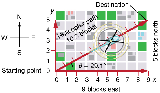
Figure 2 shows such a graphical representation of a vector, using as an example the total displacement for the person walking in a city considered in Motion in two dimensions: an introduction. We shall use the notation that an italic symbol accented by a right arrow, such as #\blue{\vec{D}}#, represents a vector. Its magnitude is represented by #\orange{\norm{D}}#, and its direction by #\green{\theta}#.
In this text, we will represent a vector with an italic variable accented by a right arrow. For example, we will represent the quantity force with the vector #\blue{\vec{F}}#, which has both magnitude and direction. The magnitude of the vector will be represented by #\orange{\norm{\vec{F}}}#, and the direction of the variable will be given by an angle #\green{\theta}#.
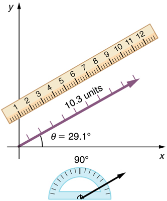
We can use a ruler and a protractor to measure a vector's magnitude and direction.
Vector addition: head-to-tail method
The head-to-tail method is a graphical way to add vectors, described in the steps below for the two displacements of the person walking in a city considered in Figure 2. The tail of the vector is the starting point of the vector, and the head (or tip) of a vector is the final, pointed end of the arrow.
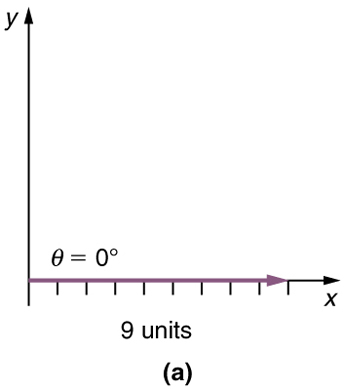
Step 1. Draw an arrow to represent the first vector (#{9}# blocks to the east) using a ruler and protractor.
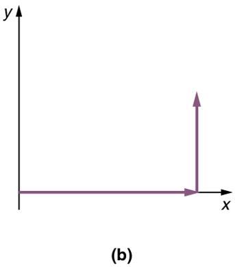
Step 2. Now draw an arrow to represent the second vector (#5# blocks to the north). Place the tail of the second vector at the head of the first vector.
Step 3. If there are more than two vectors, continue this process for each vector to be added.
Note that in our example, we have only two vectors, so we have finished placing arrows tip to tail.
Step 4. Draw an arrow from the tail of the first vector to the head of the last vector. This is the #\blue{\textbf{resultant}}#, or the sum, of the other vectors.
Step 5. To get the #\orange{\textbf{magnitude}}# of the resultant, measure its length with a ruler.
Note that in most calculations, we will use the Pythagorean theorem to determine this length.
Step 6. To get the #\green{\textbf{direction}}# of the resultant, measure its angle with the reference frame using a protractor.
Note that in most calculations, we will use trigonometric relationships to determine this angle.
The graphical addition of vectors is limited in accuracy only by the precision with which the drawings can be made and the precision of the measuring tools. It is valid for any number of vectors.
At the end of the page, we will show an example of the head-to-tail method for vector addition.
Vector subtraction
We can also subtract vectors from one another. Vector subtraction is a straightforward extension of vector addition.
Vector subtraction
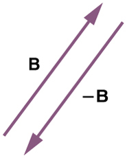
To define vector subtraction (say we want to subtract #\vec{B}# from #\vec{A}#, written #\vec{A}\ –\vec{B}#), we must first define what we mean by subtraction. The negative of a vector #\vec{B}# is defined to be #–\vec{B}#. Graphically, the negative of any vector has the same magnitude but the opposite direction as the original vector, as shown in Figure 6. In other words, #\vec{B}# has the same length as #–\vec{B}#, but points in the opposite direction. Essentially, we just flip the vector so it points in the opposite direction.
The subtraction of vector a #\vec{B}# from vector a #\vec{A}# is then simply defined to be the addition of the vector #–\vec{B}# to the vector #\vec{A}#.
Note that vector subtraction is the addition of a negative vector. The order of subtraction does not affect the results.
\[ \vec{A} \ – \vec{B} = \vec{A} +(–\vec{B})\]
and
\[\vec{A}-\vec{B}=-\vec{B}+\vec{A}\]
However, it should be noted that
\[\vec{A}-\vec{B}\ne \vec{B}-\vec{A}\]
unless #\vec{A}=\vec{B}#. This is analogous to the subtraction of scalars (where, for example, #5\ – 2 = 5 + (–2)#). Again, the result is independent of the order in which the subtraction is made. When vectors are subtracted graphically, the techniques outlined above are used, as the following example illustrates.
Multiplication of vectors and scalars
If we decided to walk three times as far on the first leg of the trip considered in the subtraction example at the end of the page, then we would walk #\purple{3}\times \unit{\orange{27.5}}{m}#, or #\unit{\orange{82.5}}{m}#, in a direction #\green{66.0^\circ}# north of east. This is an example of multiplying a vector by a positive scalar. Notice that the magnitude changes, but the direction stays the same. If the scalar is negative, then multiplying a vector by it changes the vector’s magnitude and gives the new vector the opposite direction. For example, if you multiply by #\purple{–2}#, the magnitude doubles but the direction changes.
Scalar multiplication
As seen above, when we multiply a vector by a scalar number, we obtain another vector. We can summarize the rules in the following way. When vector #\blue{\vec{A}}# is multiplied by a scalar #\purple{c}#,
- the magnitude of the vector becomes the absolute value of #\purple{c}\cdot \orange{\norm{\vec{A}}}#,
- if #\purple{c}# is positive, the direction of the vector does not change,
- if #\purple{c}# is negative, the direction is reversed.
In the case above, #\purple{c}=\purple{3}# and #\orange{\norm{\vec{A}}}=\unit{\orange{27.5}}{m}#. Vectors are multiplied by scalars in many situations. Note that division is the inverse of multiplication. For example, dividing by #\purple{2}# is the same as multiplying by #\purple{\frac{1}{2}}#. The rules for multiplication of vectors by scalars are the same for division; simply treat the divisor as a scalar between #0# and #1#.
Resolving a vector into components
In the examples above, we have been adding vectors to determine the resultant vector. In many cases, however, we will need to do the opposite. We will need to take a single vector and find what other vectors added together produce it. In most cases, this involves determining the perpendicular components of a single vector, for example the #x#- and #y#-components, or the north-south and east-west components.
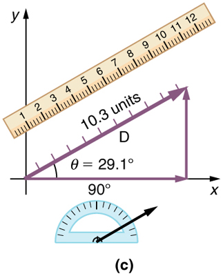
For example, we may know that the total displacement of a person walking in a city is #\orange{10.3}# blocks in a direction #\green{29.0^\circ}# north of east and want to find out how many blocks east and north had to be walked. This method is called finding the components (or parts) of the displacement in the east and north directions, and it is the inverse of the process followed to find the total displacement. It is one example of finding the components of a vector. There are many applications in physics where this is a useful thing to do. We will see this soon in Projectile motion I and II, and much more when we cover forces in Dynamics: Newton’s laws of motion. Most of these involve finding components along perpendicular axes (such as north and east), so that right triangles are involved. The analytical techniques presented in Vector addition and subtraction: analytical methods are ideal for finding vector components.
Adding vectors graphically using the head-to-tail method: a woman takes a walk
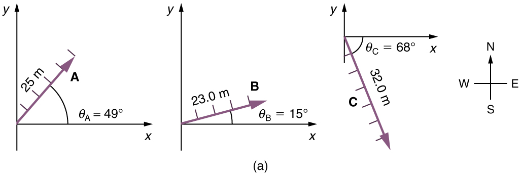
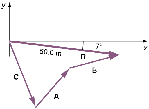
Use the graphical technique for adding vectors to find the total displacement of a person who walks the following three paths (displacements) on a flat field. First, she walks #\unit{25.0}{m}# in a direction #49.0^\circ# north of east. Then, she walks #\unit{23.0}{m}# heading #15.0^\circ# north of east. Finally, she turns and walks #\unit{32.0}{m}# in a direction #68.0^\circ# south of east.
1. Outline the strategy
Represent each displacement vector graphically with an arrow, labeling the first #\vec{A}#, the second #\vec{B}#, and the third #\vec{C}#, making the lengths proportional to the distance and the directions as specified relative to an east-west line. The head-to-tail method outlined above will give a way to determine the magnitude and direction of the resultant displacement, denoted #\vec{R}#.
2. Head-to-tail method for vector addition
(1) Draw the three displacement vectors.
(2) Place the vectors head to tail retaining both their initial magnitude and direction.
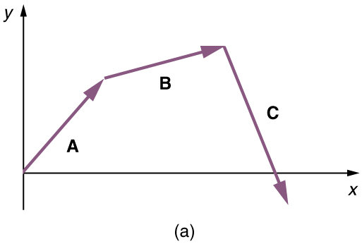
(3) Draw the resultant vector, #\vec{R}#.
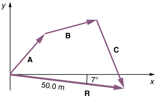
(4) Use a ruler to measure the magnitude of #\vec{R}#, and a protractor to measure the direction of #\vec{R}#. While the direction of the vector can be specified in many ways, the easiest way is to measure the angle between the vector and the nearest horizontal or vertical axis. Since the resultant vector is south of the eastward pointing axis, we flip the protractor upside down and measure the angle between the eastward axis and the vector.
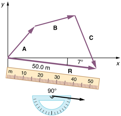
In this case, the total displacement #\vec{R}# is seen to have a magnitude of #\unit{50.0}{m}# and to lie in a direction #7.0^\circ# south of east. By using its magnitude and direction, this vector can be expressed as #R=\unit{50.0}{m}# and #\theta =7.0^\circ# south of east.
Discussion
The head-to-tail graphical method of vector addition works for any number of vectors. It is also important to note that the resultant is independent of the order in which the vectors are added. Therefore, we could add the vectors in any order as illustrated in the figure below and we will still get the same solution.
Here, we see that when the same vectors are added in a different order, the result is the same. This characteristic is true in every case and is an important characteristic of vectors. Vector addition is commutative. Vectors can be added in any order.
\[\vec{A}+\vec{B} = \vec{B}+\vec{A}\]
This is true for the addition of ordinary numbers as well. You get the same result whether you add #{2}+{3}# or #{3}+{2}#, for example.