Accuracy, precision, and significant figures

[OpenStax, College physics 2e, Introduction: the nature of science and physics] The nature of science and physics: Physics: an introduction

Accuracy, precision, and significant figures

Accuracy, precision, and uncertainty of a measurement

Accuracy and precision are often used interchangeably in everyday use. However their difference is quite important.

Accuracy and precision

Science is based on observation and experiment, that is, on measurements. Accuracy is how close a measurement is to the correct value for that measurement.

The precision of a measurement system refers to how close the agreement is between repeated measurements (which are repeated under the same conditions).

Example: piece of paper

For example, let us say that you are measuring the length of a standard sheet of A4 paper. The packaging in which you purchased the paper states that it is #29.7# centimeters long. You measure the length of the paper three times and obtain the following measurements: #\unit{29.5}{cm}#, #\unit{29.6}{cm}#, and #\unit{30.0}{cm}#. These measurements are quite accurate because they are very close to the correct value of #29.7# centimeters. In contrast, if you had obtained a measurement of #32# centimeters your measurement would not be very accurate.

The precision of the measurements refers to the spread of the measured values. One way to analyze the precision of the measurements would be to determine the range, or difference, between the lowest and the highest measured values. In that case, the lowest value was #\unit{29.5}{cm}# and the highest value was #\unit{30.0}{cm}# Thus, the measured values deviated from each other by at most #\unit{0.5}{cm}#. These measurements were relatively precise because they did not vary too much in value. However, if the measured values had been #\unit{29.1}{cm}#, #\unit{28.3}{cm}#, and #\unit{31.7}{cm}#, then the measurements would not be very precise because there would be significant variation from one measurement to another.

Example: accurate, precise, both, or neither

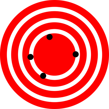
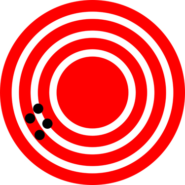
The measurements in the paper example are both accurate and precise, but in some cases, measurements are accurate but not precise, or they are precise but not accurate. Let us consider an example of a GPS system that is attempting to locate the position of a restaurant in a city. Think of the restaurant location as existing at the center of a bull’s-eye target, and think of each GPS attempt to locate the restaurant as a black dot. In Figure 1, you can see that the GPS measurements are spread out far apart from each other, but they are all relatively close to the actual location of the restaurant at the center of the target. This indicates a low precision, high accuracy measuring system. However, in Figure 2, the GPS measurements are concentrated quite closely to one another, but they are far away from the target location. This indicates a high precision, low accuracy measuring system.

Fig. 1 A GPS system attempts to locate a restaurant at the center of the bull’s-eye. The black dots represent each attempt to pinpoint the location of the restaurant. The dots are spread out quite far apart from one another, indicating low precision, but they are each rather close to the actual location of the restaurant, indicating high accuracy (credit: Dark Evil).

Fig. 2 In this figure, the dots are concentrated rather closely to one another, indicating high precision, but they are rather far away from the actual location of the restaurant, indicating low accuracy (credit: Dark Evil).

Regarding accuracy and precision, it is useful to be able to state how certain we are about a measurement. To do so, we need the concept of uncertainty.

Uncertainty

The degree of accuracy and precision of a measuring system are related to the uncertainty in the measurements. Uncertainty is a quantitative measure of how much your measured values deviate from a standard or expected value.

If your measurements are not very accurate or precise, then the uncertainty of your values will be very high. In more general terms, uncertainty can be thought of as a disclaimer for your measured values. All measurements contain some amount of uncertainty.

The uncertainty in a measurement, #\blue{A}#, is often denoted as #\green{\delta A \text{ (“delta $ A$”)}}#, so the measurement result would be recorded as #\blue{A}\pm\green{\delta A}#.

Example

For example, if someone asked you to provide the mileage on your car, you might say that it is #\blue{80000}# kilometers, plus or minus #\green{1000}# kilometers. The plus or minus amount is the uncertainty in your value. That is, you are indicating that the actual mileage of your car might be as low as #\blue{79000}# kilometers or as high as #\blue{81000}# kilometers, or anywhere in between.

Example: piece of paper

In our example of measuring the length of the paper, we might say that the length of the paper is #\blue{\unit{29.7}{cm}}#, plus or minus #\green{\unit{0.4}{cm}}#. This could be expressed as #\unit{\blue{29.7}\pm \green{0.4}}{\green{cm}}#

Factors contributing to the uncertainty could be the following: the smallest division on the ruler is #\unit{0.1}{cm}#, the person using the ruler has bad eyesight, or one side of the paper is slightly longer than the other. At any rate, the uncertainty in a measurement must be based on a careful consideration of all the factors that might contribute and their possible effects.

Fevers or chills?

Uncertainty is a critical piece of information, both in physics and in many other real-world applications. Imagine you are caring for a sick child. You suspect the child has a fever, so you check his or her temperature with a thermometer. What if the uncertainty of the thermometer were #\green{\unit{3.0}{^\circ C}}#? If the child’s temperature reading was #\blue{\unit{37.0}{^\circ C}}# (which is normal body temperature), the “true” temperature could be anywhere from a hypothermic #\blue{\unit{34.0}{^\circ C}}# to a dangerously high #\blue{\unit{40.0}{^\circ C}}#. A thermometer with an uncertainty of #\green{\unit{3.0}{^\circ C}}# would be useless.

The factors contributing to uncertainty in a measurement include:

limitations of the measuring device,
the skill of the person making the measurement,
irregularities in the object being measured,
any other factors that affect the outcome (highly dependent on the situation).

The uncertainty can also be expressed relative to the measured value.

Percent uncertainty

One method of expressing uncertainty is as a percent of the measured value. If a measurement #\blue{A}# is expressed with uncertainty, #\green{\delta A}#, the percent uncertainty (#\orange{\%\text{unc} }#) is defined to be

\[ \orange{\%\text{unc}} =\dfrac{\green{\delta A}}{\blue{A}}\cdot 100\%\]

Uncertainties in calculations

There is an uncertainty in anything calculated from measured quantities. For example, the area of a floor calculated from measurements of its length and width has an uncertainty because the length and width have uncertainties. How big is the uncertainty in something you calculate by multiplication or division? If the measurements going into the calculation have small uncertainties (a few percent or less), then the method of adding percents can be used for multiplication or division.

This method says that the percent uncertainty in a quantity calculated by multiplication or division is the sum of the percent uncertainties in the items used to make the calculation.

For example, if a floor has a length of #\blue{\unit{4.00}{m}}# and a width of #\blue{\unit{3.00}{m}}#, with uncertainties of #\orange{2\%}# and #\orange{1\%}#, respectively, then the area of the floor is #\blue{\unit{12.0}{m^2}}# and has an uncertainty of #\orange{3\%}#. Expressed as an area this uncertainty is #\green{\unit{0.36}{m^2}}#, which we round to #\green{\unit{0.4}{m^2}}# since the area of the floor is given to a tenth of a square meter.

Calculating percent uncertainty: a bag of apples

A grocery store sells #\blue{\unit{5}{kg}}# bags of apples. You purchase four bags over the course of a month and weigh the apples each time. You obtain the following measurements:

week 1 weight: #\blue{\unit{4.8 }{kg}}#,
week 2 weight: #\blue{\unit{5.3 }{kg}}#,
week 3 weight: #\blue{\unit{4.9 }{kg}}#,
week 4 weight: #\blue{\unit{5.4 }{kg}}#.

You determine that the weight of the #\blue{\unit{5}{kg}}# bag has an uncertainty of #\green{\pm \unit{0.4}{kg}}#. What is the percent uncertainty of the bag’s weight?

1. Outline a strategy

First, observe that the expected value of the bag’s weight, #\blue{A}#, is #\blue{ \unit{5}{kg}}#. The uncertainty in this value, #\green{\delta A}#, is #\green{\unit{0.4}{kg}}#. We can use the following equation to determine the percent uncertainty of the weight:

\[\orange{\%\text{unc}} =\dfrac{\green{\delta A}}{\blue{A}}\cdot 100\%\]

2. Solve for percent uncertainty

We just have to fill in the numerical values in the equation above.
\[\begin{array}{rcl}
\orange{\%\text{unc}} &=&\dfrac{\green{\delta A}}{\blue{A}}\cdot 100\%\\
&&\quad \blue{\text{formula for the percent uncertainty}}\\
&=&\dfrac{\green{0.4}}{\blue{5}}\cdot 100\%\\
&&\quad \blue{\text{filled in the numerival values}}\\
&=&\orange{8\%}\\
&&\quad \blue{\text{computed}}
\end{array}\]

Discussion

We can conclude that the weight of the apple bag is #\blue{\unit{5}{kg}} \pm \orange{8\%}#. Consider how this percent uncertainty would change if the bag of apples were half as heavy, but the uncertainty in the weight remained the same. Hint for future calculations: when calculating percent uncertainty, always remember that you must multiply the fraction by #100\%#. If you do not do this, you will have a decimal quantity, not a percent value.

New example

Fig. 3 A double-pan mechanical balance is used to compare different masses. Usually an object with unknown mass is placed in one pan and objects of known mass are placed in the other pan. When the bar that connects the two pans is horizontal, then the masses in both pans are equal. The “known masses” are typically metal cylinders of standard mass such as #1# gram, #10# grams, and #100# grams (credit: Serge Melki).

Fig. 4 Many mechanical balances, such as double-pan balances, have been replaced by digital scales, which can typically measure the mass of an object more precisely. Whereas a mechanical balance may only read the mass of an object to the nearest tenth of a gram, many digital scales can measure the mass of an object up to the nearest thousandth of a gram (credit: Karel Jakubec).

Precision of measuring tools and significant figures

An important factor in the accuracy and precision of measurements involves the precision of the measuring tool. In general, a precise measuring tool is one that can measure values in very small increments. For example, a standard ruler can measure length to the nearest millimeter, while a caliper can measure length to the nearest #\green{0.01}# millimeter. The caliper is a more precise measuring tool because it can measure extremely small differences in length. The more precise the measuring tool, the more precise and accurate the measurements can be.

When we express measured values, we can only list as many digits as we initially measured with our measuring tool. For example, if you use a standard ruler to measure the length of a stick, you may measure it to be #\blue{\unit{36.7}{cm}}#. You could not express this value as #\blue{\unit{36.71}{cm}}# because your measuring tool was not precise enough to measure a hundredth of a centimeter. It should be noted that the last digit in a measured value has been estimated in some way by the person performing the measurement.

For example, the person measuring the length of a stick with a ruler notices that the stick length seems to be somewhere in between #\blue{\unit{36.6}{cm}}# and #\blue{\unit{36.7}{cm}}#, and he or she must estimate the value of the last digit.

Significant figures

Using the method of significant figures, the rule is that the last digit written down in a measurement is the first digit with some uncertainty. In order to determine the number of significant digits in a value, start with the first measured value at the left and count the number of digits through the last digit written on the right. For example, the measured value #\blue{\unit{36.7}{cm}}# has three digits, or significant figures. Significant figures indicate the precision of a measuring tool that was used to measure a value.

It is particularly important to consider how to count the #0# digit depending on the context where it appears.

Zeros

Special consideration is given to zeros when counting significant figures. The zeros in #0.053# are not significant, because they are only placekeepers that locate the decimal point. There are two significant figures in #0.053#.

The zeros in #10.053# are not placekeepers but are significant. This number has five significant figures.

The zeros in #1300# may or may not be significant depending on the style of writing numbers. They could mean the number is known to the last digit, or they could be placekeepers. So #1300# could have two, three, or four significant figures. To avoid this ambiguity, write #1300# in scientific notation.

Zeros are significant except when they serve only as placekeepers.

When combining measurements with different degrees of accuracy and precision, the number of significant digits in the final answer can be no greater than the number of significant digits in the least precise measured value. There are two different rules, one for multiplication and division and the other for addition and subtraction, as discussed below.

Significant figures in calculations

For multiplication and division the result should have the same number of significant figures as the quantity having the least significant figures entering into the calculation.

For addition and subtraction the answer can contain no more decimal places than the least precise measurement.

Example multiplication and division

For example, the area of a circle can be calculated from its radius using #A=\pi\cdot r^{2}#. Let us see how many significant figures the area has if the radius has only two. Suppose we measure #r=\blue{\unit{1.2}{m}}#, the area would be:

\[ \begin{array}{rcl}
A&=&\pi\cdot r^{2}\\
&&\quad \blue{\text{formula for the area of a circle}}\\
&=&(3.1415927...)\cdot {(\blue{1.2})}^{2}\\
&&\quad \blue{\text{filled in the numerical values}}\\
&=&\blue{\unit{4.5238934}{m^2}}\\
&&\quad \blue{\text{computed}}
\end{array}\]

This last value is what you would get using a calculator that has an eight-digit output. But because the radius has only two significant figures, it limits the calculated quantity to two significant figures even though #\pi # is good to at least eight digits:

\[ A=\blue{\unit{4.5}{m^2}}\]

Example addition and subtraction

Suppose that you buy #\blue{\unit{7.56}{kg}}# of potatoes in a grocery store as measured with a scale with precision #\green{\unit{0.01}{kg}}#. Then you drop off #\blue{\unit{6.052}{kg}}# of potatoes at your laboratory as measured by a scale with precision #\green{\unit{0.001}{kg}}#. Finally, you go home and add #\blue{\unit{13.7}{kg}}# of potatoes as measured by a bathroom scale with precision #\green{\unit{0.1}{kg}}#. How many kilograms of potatoes do you now have, and how many significant figures are appropriate in the answer? The mass is found by simple addition and subtraction:

\[\begin{array}{rcl}
\blue{\unit{7.56\phantom{0}}{kg}} &&\\
\blue{\unit{-\;\phantom{1}6.052}{kg}} &&\\
\blue{\underline{\unit{+\;13.7\phantom{00}}{kg}}}&&\\
\blue{\unit{15.208}{kg} }&=&\blue{\unit{15.2}{kg}}
\end{array}\]

Next, we identify the least precise measurement: #\blue{\unit{13.7}{kg}}#. This measurement is expressed to the #0.1# decimal place, so our final answer must also be expressed to the #0.1# decimal place. Thus, the answer is rounded to the tenth place, giving us #\blue{\unit{15.2}{kg}}#.

Exact numbers

If a number is exact, such as the two in the formula for the circumference of a circle, #c=2\cdot\pi \cdot r#, it does not affect the number of significant figures in a calculation.

Significant figures in this text

In most exercises, we will ask for answers with three significant figures and give data with three to four significant figures. Due to ambiguities in rounding, intermediate results will often be displayed with four significant figures. When the exercise requires computing the value of a trigonometric function, we will display the associated steps with five significant figures.